Mother’s Day
Jimboy wishes that he was created in a mechanical uterus so that his dad could pay for the machine to end the constant nagging by mom for carrying him for nine months. However, most mothers and their off springs have better relationships and celebrate Mother’s Day. Sara and Johnny had previously collected data on the average expenditure by sons/daughters on Mother’s Day for the years 2009-2019. Although a year had gone by the two starting chatting about it when Johnny found the data on his laptop.
| Expenditure in Dollars | |||||
| Year | Year minus- 2009 | Mother’s Day | Father’s Day | Valentine’s Day | |
| 2009 | 0 | 123.89 | 81.71242 | 103 | |
| 2010 | 1 | 126.9 | 85.18954 | 103 | |
| 2011 | 2 | 140.73 | 96.4902 | 116 | |
| 2012 | 3 | 152.52 | 110.3987 | 126 | |
| 2013 | 4 | 168.94 | 115.6144 | 131 | |
| 2014 | 5 | 162.98 | 108.6601 | 134 | |
| 2015 | 6 | 172.63 | 110.3987 | 142 | |
| 2016 | 7 | 172.22 | 124.3072 | 147 | |
| 2017 | 8 | 186.39 | 134.7386 | 137 | |
| 2018 | 9 | 179.77 | 133 | 144 | |
| 2019 | 10 | 196.47 | 138 | 162 |
Straight Line
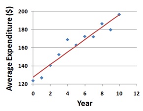
Sara: The average expenditure per person on Mother’s Day increased with time as we found before.
Johnny took a ruler and drew a line over the data points and said: Yes, it looks like a linear relationship of the expenditure with time. It has a positive slope showing that the expenditure increased with time. I took the year 2009 to be the year zero since we do not have any data before this time.
Sara: I like the way you just took a ruler and drew a line between the points. How do you know that this is the best fit line for these data ?
Johnny: What do you mean ? Looks good to me. How else would you do it ?
Linear regression
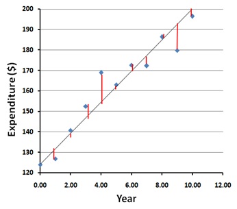
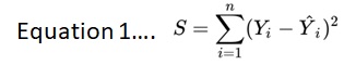
Sara: Here, I draw red lines between the actual values of expenditures (Yi) and the values based on the line you drew (Y^i). The lengths of these lines (Yi – Y^i) show how these values deviate from the line. Since the squares of these lengths will all be positive, the best fit would result in minimum value of the sum of (Yi-Y^i)2 for the 11 years (n) of the data. We can write this sum S as equation 1.
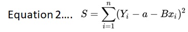
Since the equation of a straight line is Y = a + Bx, where a is the Y- intercept and B is the slope, we can write it as equation 2.
Johnny: I like the way you bring calculus into everything. Now this is a minimization problem. I think it will involve at least three concepts – first derivative has to be zero for a minima, partial differentials because you have to minimize with respect to a and B, and may be also the chain rule.
Sara: Shows how well I taught you calculus and also that you got an A+ in the course, smart guy.
Johnny: Let us go with the partial derivative ∂S/∂a = 0 first as in the equations 3, 4 and 5.
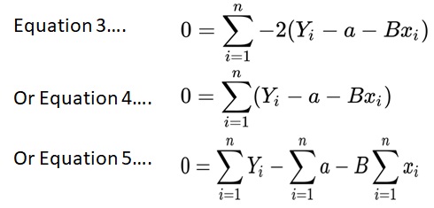
Now sum of all values of a from 1 to n is na, therefore a will be given by equation 6.
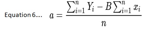
which is the same as na = (n meanYi – B n mean xi) or a = (mean Yi – B mean xi).
Next we will go with the derivative ∂S/∂B = 0 starting with equation 7.
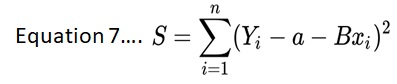
Using the chain rule ∂S/∂B = 0 becomes equation 8 and then equation 9.
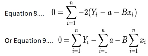
Now sum of all values of a from 1 to n is na, and a = (Yi mean -B mean xi). Therefore, we can write equations 10, 11 and 12.
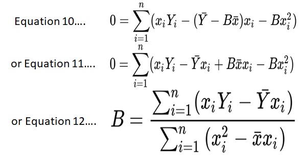
This way, we can determine the slope and the intercept for the line of best fit. This is the formula most calculators and computer software are based on.
Johnny: So you mean, we can either calculate the least square regression line with these formulas or with a computer program. I am going to use Excel to calculate the slope and the intercept and graph the line.
Sara: What values did you have for the y-intercept and the slope ?
Johnny: The Y-intercept was 127.84 and the slope was 6.86. That means that each person spends on average $6.86 more than the previous year.
Sara: Great, now we can compare this with the expenditures on Father’s Day and Valentine’s Day.
| Mother’s Day | Father’s Day | Valentine Day | |
| Y-intercept | 127.84 | 84.86 | 105.83 |
| Slope | 6.86 | 5.55 | 5.23 |
Johnny: Looks like, mothers win all the way. The average expenditure on mother’s day ($127.84) is the largest of the three in 2009 and increased at a higher rate ($6.86 per year) than the other two.
Sara: Yes, the average expenditure of the Valentine’s Day ($105.83) was slightly higher in 2009 than on the Father’s Day ($84.86) but both increased at very similar rates over the years.
Note, it is also possible to determine the errors in these parameters and then determine their levels of confidence (reliability) but these will are left for statistics courses.
Challenge
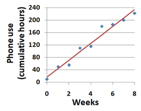
Joey’s father scolded him for being on the phone all the time. He told him to record hours of phone use each week and show him a trend line. Joey recorded the hours as shown in the Table and thought that the cumulative phone use/week should be a straight line. What should he do next ?
Solution: He should carry out linear regression. Doing so with Microsoft program Excel gave a Y-intercept of 16.9 and a slope of 27.1.
Based on that he should calculate points for the line of best fit with the formula
Y = Yintercept + weeks x slope
Best fit hours = 16.9 + weeks x 27.1 as shown in the table. Then he should graph them to show values of Yi and the line of best fit as shown in the graph.
| Joey’s Phone Use Record | ||
| Week | Cumulative Use (hours) | Best Fit Line |
| 0 | 10 | 16.9 |
| 1 | 50 | 44 |
| 2 | 55 | 71.1 |
| 3 | 110 | 98.2 |
| 4 | 115 | 125.3 |
| 5 | 180 | 152.4 |
| 6 | 185 | 179.5 |
| 7 | 200 | 206.6 |
| 8 | 222 | 233.7 |